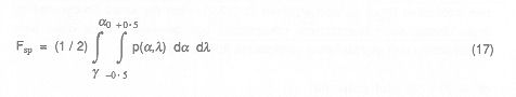
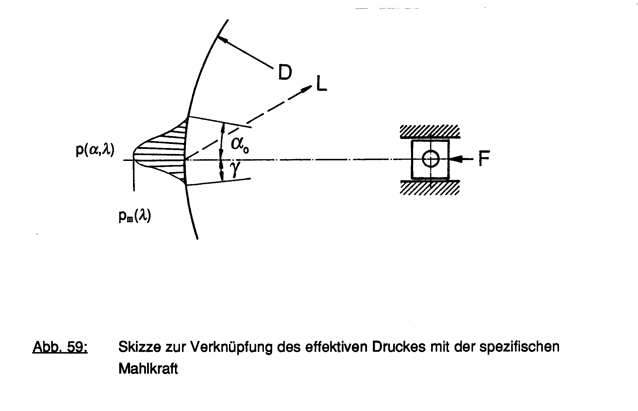
For the calculation of the integral p(a,l) as well as a₀ and g must be known. A difficulty is that a₀ and g may principally depend on l and F_sp. Nevertheless the tests have shown only weak dependencies. Therefore in the following the independency of  l and F_sp is assumed. The tests also show - and it will be proven later - that the pressure distribution can be expressed as an approximation by a product of two one-parametrical functions. Then the double integral  can be transformed into a product of two single integrals:

p(a,l) =  p_m(l)  f(a)                                                                             (18)

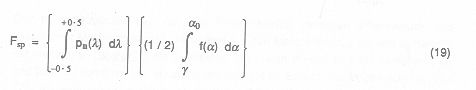
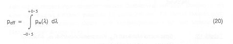
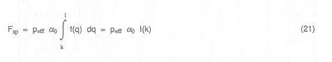
The first integral is the determination equation for the effective pressure p_eff:

Of course the axial pressure distribution is impacted by the relations of roller length to roller diameter, roller diameter to particle size and the geometrical situation at the roller edge. The effective pressure is therefore principally depending on those parameters:

p_eff = p_eff(L/D, D/x, edge)

These influences are still unknown and need further investigation.

At this point the normalized angle coordinate q = a/a₀ is introduced and the relation (g/a₀) is named k. With these definitions it follows:

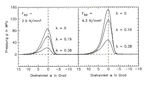
With this transformation we have an equation to determine the integral expression.

I(k) = F_sp / p_eff a₀

As a conclusion the integral expression I(k) which characterizes the proportionality between effective pressure and specific grinding force can be calculated from the measured parameters p_eff ,F_sp and a₀, see table with calculated values of I(k).With exception of the first value I(k) lies between 0.26 and 0.30, is therefore almost constant and fits well into the the range given by the calculation modell in [2]. A possible explanation for the higher value of 0.40 for the quartz fraction and the smallest specific grinding force of 1.5 N/mm² can be given by the bigger pressure measurement variations and the smaller number of pressure measurements. High Compression Roller Mills are usually working with specific grinding force between 2.5 and 6.0 N/mm². For this range a value of I(k) results which is independent of material and particle size for the tested quartz and limestone fractions.

To prove that the splitting of the pressure distribution p(a,l) according equation (18) is allowed the preipheral pressure distributions of the tests with limestone fractions 1.2/1.8 mm are used, see following diagrams. Out of the six measured pressure distributions

p(a, l_i, F_sp,j)            with l₁ = 0 / l₂ = 0.19 / l₃ = 0.38                                                                        as well as F_sp,1 = 2.9 N/mm² and F_sp,2 = 4.3 N/mm²

the integral average values are calculated in a first step:

Averaged pressure diagrams in three different roller layers for limestone 1.2/1.8 mm, u = 0.3 m/s.

With these the averaged average can be calculated

and the normalizing factors t_i,j:

With this the following normalized pressure distributions can be calculated

which are shown in the following diagram.

Normalized pressure diagrams for two specific grinding forces and in three different roller layers each, for limestone 1.2/1.8 mm, u = 0.3 m/s.

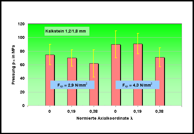
In fact some tendencies can be seen (e.g. pressure distribution at l = 0.38 slightly above the others) but the confidence intervals for the previously discussed statistical variations on a probability of error level of 5 % are overlapping, see following diagram. Therefore the required precondition that p(a,l) =  p_m(l)  f(a) can be seen as fulfilled.

95 %-confidence intervalsfor the normalized pressure distributions above